Data Post Processing#
In this tutorial we will do the following#
Download ERA5 precipitation data from Amazon S3 using earth2observe.
Change the format of the downloaded data from netcdf to rasters each represent one time stamp.
Create Index map, to refer to the location of each cell with an index number.
Create point (at the center of the cell) and polygon (covers the whole cell) geometries to use also as an index.
Convert the rasters into columns in a dataframe.
Use Uber H3 spatial index to get the spatial index for all cells for all 16 resolution.
- WE will be using
earth2observe package
The convert module in the Pyramids package (dependency of earth2observe you don’t need to install it separately)
- Tutorial notebook
- You don’t need to copy and paste the code snippts in this tutorial, you can find the whole tutorial as a
jupyter notebook post processing of ERA5 data.
Packages#
you only need to install earth2observe from conda-forge
conda install -c conda-forge earth2observe=0.2.2
or from pip
pip install earth2observe==0.2.2
Import packages
import os
import glob
import datetime as dt
from loguru import logger
import geopandas as gpd
import pandas as pd
from pyramids.raster import Raster
from pyramids.convert import Convert
from osgeo import gdal
from osgeo.gdal import Dataset
import numpy as np
from pyramids.indexing import H3
from earth2observe.earth2observe import Earth2Observe
Setup#
First define the root directory where all the data will be stored
rdir = "project"
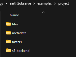
The directory should have 4 folders
project
files
metadata
rasters
s3-backend
- files:
Contains the processed data saved in a parquet format
- metadata: contains 3 files
index.tif: index raster.
index_points.parquet: index point geometry.
index_polygon.parquet: index polygon geometry.
- rasters:
Cotains the 1-band raster files converted from the downloaded netcdf, each raster represent 1 time step in the downloaded data time series.
- s3-backend:
Contains the downloaded netcdf files.
Earth2observe abstract class#
Second define the earth2observe parameters.
- data_source: [str]
data source name. the available data sources are [“ecmwf”, “chirps”, “amazon-s3”].
- temporal_resolution (str, optional):
temporal resolution. Defaults to ‘daily’.
- start (str, optional):
start date. Defaults to ‘’.
- end (str, optional):
end date. Defaults to ‘’.
- path (str, optional):
Path where you want to save the downloaded data. Defaults to ‘’.
- variables (list, optional):
Variable name.
- lat_lim (list, optional):
[ymin, ymax]. Defaults to None.
- lon_lim (list, optional):
[xmin, xmax]. Defaults to None.
- fmt (str, optional):
date format. Defaults to “%Y-%m-%d”.
start = "2022-05-01"
end = "2022-05-01"
time = "monthly"
path = f"{rdir}/s3-backend"
source = "amazon-s3"
variables = ["precipitation"]
e2o = Earth2Observe(
    data_source=source,
    temporal_resolution=time,
    start=start,
    end=end,
    path=path,
    variables=variables,
)

e2o.download()

Post processing#
- Convert the downloaded netcdf into rasters one for each time stamp in the ncdf file For the example I converted only
1-hourly rasters.
nc_file = f"{path}/202205_monthly_precipitation_amount_1hour_Accumulation.nc"
save_to = f"{rdir}/rasters"
Convert.nctoTiff(nc_file, save_to, time_var_name="time1", prefix="Amazon-S3-ERA5")
In this part we will create a spatial index for each cell in the downloaded rasters, and convert the rasters into a pandas dataframe.
- First spatial indexing method, we will create an index raster with an id for each cell that will refer to the row in
the dataframe to be able to locate the value and associate it to a specific location.
- Second method we will create a point/polygon geometry at the center of each cell so we can query the whole raster but
using geometries relations. for more information on how the rasterToGeoDataFrame function works, please check the documentation of the pyramids package rasterToGeoDataFrame documentation .
- Third we will use the H3 indexing method so we can assign a hexadecimal index (for each resolution 0-15) so we can
use the different resolution of H3 tfor faster querying of data. for more information H3 Documentation.
- The creation of the polygon index will take a bit long time (3 min) but it is optional since we can only use the
point index.
So the point/polygon and raster index will be created only once since all rasters have the same dimensions.
- After converting all rasters into a dataframe ewe will use the point index to get the H3 index for all points for
the 16 resolutions and add them to the same dataframe.
In the last step we will save the dataframe as a parquet data type.
- In the following function we defined all the above steps and we will call the function and use one of the rasters in
the rasters folder
from osgeo.gdal import Dataset

def create_metadata(src: Dataset, path: str):
    """Create the index raster and the geometry file (both point and polygon)

    Parameters
    ----------
    src: [Dataset]
        gdal Dataset.
    path: [str]
        path to where the metadata are going to be saved.
    """
    # first create the raster
    logger.info("First step (creating index raster)")
    arr = src.ReadAsArray()
    rows, cols = arr.shape

    unique_nums = list(range(1, rows * cols + 1))
    arr = np.array(unique_nums)
    new_arr = np.reshape(arr, (rows, cols))
    dst= Raster.rasterLike(src, new_arr, driver="MEM")
    Raster.saveRaster(dst, f"{path}/index.tif")
    # second create the point index file from the index raster
    logger.info("Second step (Create index point geometry file)")
    logger.info("The Point geometry will be created at the center of each cell so we can query the cells values by "
                "indexing the cell center location")
    logger.info("This step might take couple of minutes but these step are executed only once to create the metadata")
    gdf = Convert.rasterToGeoDataFrame(dst, add_geometry="point")
    gdf.to_parquet(f"{path}/index_points.parquet", index=False, compression='gzip')
    # third create the polygon index file from the index raster
    logger.info("Third step (Create index polygon geometry file)")
    gdf = Convert.rasterToGeoDataFrame(dst, add_geometry="polygon")
    gdf.to_parquet(f"{path}/index_polygon.parquet", index=False, compression='gzip')
    logger.info("Creating index data has finished successfully")
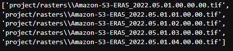
using glob we will get all the rasters in the rasters folder.
search_criteria = "*.tif"
file_list = glob.glob(os.path.join(f"{rdir}/rasters", search_criteria))
print(file_list)
Now we will call the create_metadata function we created above.
fname = file_list[0]
src = gdal.Open(fname)
meta_data_path = f"{rdir}/metadata"
create_metadata(src, meta_data_path)

>>> 2023-01-29 05:36:11.662 | INFO     | __main__:create_metadata:14 - First step (creating index raster)
>>> 2023-01-29 05:36:11.746 | INFO     | __main__:create_metadata:24 - Second step (Create index point geometry file)
>>> 2023-01-29 05:36:11.747 | INFO     | __main__:create_metadata:25 - The Point geometry will be created at the center of each cell so we can query the cells values by indexing the cell center location
>>> None
>>> 2023-01-29 05:37:37.518 | INFO     | __main__:create_metadata:30 - Third step (Create index polygon geometry file)
>>> 2023-01-29 05:39:18.811 | INFO     | __main__:create_metadata:33 - Creating index data has finished successfully
Convert the downloaded data into dataframes.#
In this part we will convert the rasters into Dataframe using the convert module in the Pyramids package.
- The Pyramids package is a GIS utility package that handles raster and vector data in addition to multiple other
dataformat.
- In the convert module in the pyramids package there are couple of function that can convert data from format to
another like rasterToPolygon, polygonToRaster, and rasterToGeoDataFrame.
- For more information on how the rasteToGeodataFrame function works you can check the
rows = src.RasterYSize
cols = src.RasterXSize
fmt = "%Y.%m.%d.%H.%M.%S"
hourly_fmt = "%Y-%m-%d-%H"
data = np.zeros(shape=(rows * cols, len(file_list))) * np.nan
file_order = []
for i, fname in enumerate(file_list):
    date_fragments = fname.split("_")[-1][:-4]
    file_order.append(dt.datetime.strptime(date_fragments, fmt))
    data[:, i] = Convert.rasterToGeoDataFrame(fname).values.reshape((rows*cols))

col_names = [date_i.strftime(hourly_fmt) for date_i in file_order]
# making the date as an index makes the files size grows drastically
df = pd.DataFrame(data, columns=col_names)
df.to_parquet(f"{rdir}/files/data.parquet", index=False, compression='gzip')
Now we can check the df to see what is stored there.
print(df.head())
>>> 2022-05-01-00   2022-05-01-01   2022-05-01-02   2022-05-01-03   2022-05-01-04
>>> 0       0.000061        0.0     0.0     0.000061        0.000122
>>> 1       0.000061        0.0     0.0     0.000061        0.000122
>>> 2       0.000061        0.0     0.0     0.000061        0.000122
>>> 3       0.000061        0.0     0.0     0.000061        0.000122
>>> 4       0.000061        0.0     0.0     0.000061        0.000122
Indexing the data with h3#
Read the parquet file containing the extracted cell values and generating the H3 index for each resolution level.
df = pd.read_parquet(f"{rdir}/files/data.parquet")
# read the point index file and index
point_index = gpd.read_parquet(f"{rdir}/metadata/index_points.parquet")
print("Extract the coordinates from each point in the point index geometry file we created in the last step to use it in obtaining the h3 index for different resolutions")
coords = [(i.x, i.y) for i in point_index["geometry"]]

for res in range(16):
    print(f"H3 resolution :{res}")
    hex = [H3.geometryToIndex(xy[1], xy[0], res) for xy in coords]
    # hex = H3.getIndex(point_index, res)
    df[f"{res}"] = hex

df.to_parquet(f"{rdir}/files/data.parquet", index=False, compression='gzip')

>>> H3 resolution :0
>>> H3 resolution :1
>>> H3 resolution :2
>>> H3 resolution :3
>>> H3 resolution :4
>>> H3 resolution :5
>>> H3 resolution :6
>>> H3 resolution :7
>>> H3 resolution :8
>>> H3 resolution :9
>>> H3 resolution :10
>>> H3 resolution :11
>>> H3 resolution :12
>>> H3 resolution :13
>>> H3 resolution :14
>>> H3 resolution :15
Now all the preprocessing tasks is done and you have the data saved in the parquet data format, we can read it and query it.
df = pd.read_parquet(f"{rdir}/files/data.parquet")
print(df.head())

>>> 2022-05-01-00   2022-05-01-01   2022-05-01-02   2022-05-01-03   2022-05-01-04   0       1       2       3       4       ...     6       7       8       9       10      11      12      13      14      15
>>> 0       0.000061        0.0     0.0     0.000061        0.000122        80f3fffffffffff 81f2bffffffffff 82f297fffffffff 83f293fffffffff 84f2939ffffffff ...     86f293957ffffff 87f293956ffffff 88f293956bfffff 89f293956afffff 8af293956ac7fff 8bf293956ac2fff 8cf293956ac23ff 8df293956ac223f 8ef293956ac2237 8ff293956ac2234
>>> 1       0.000061        0.0     0.0     0.000061        0.000122        80f3fffffffffff 81f2bffffffffff 82f297fffffffff 83f293fffffffff 84f2939ffffffff ...     86f293957ffffff 87f293956ffffff 88f293956bfffff 89f293956afffff 8af293956ac7fff 8bf293956ac3fff 8cf293956ac33ff 8df293956ac337f 8ef293956ac3347 8ff293956ac3341
>>> 2       0.000061        0.0     0.0     0.000061        0.000122        80f3fffffffffff 81f2bffffffffff 82f297fffffffff 83f293fffffffff 84f2939ffffffff ...     86f293957ffffff 87f293956ffffff 88f293956bfffff 89f293956afffff 8af293956acffff 8bf293956ac8fff 8cf293956ac8dff 8df293956ac8c3f 8ef293956ac8c17 8ff293956ac8c15
>>> 3       0.000061        0.0     0.0     0.000061        0.000122        80f3fffffffffff 81f2bffffffffff 82f297fffffffff 83f293fffffffff 84f2939ffffffff ...     86f293957ffffff 87f293956ffffff 88f293956bfffff 89f293956afffff 8af293956acffff 8bf293956ac9fff 8cf293956ac9dff 8df293956ac9d7f 8ef293956ac9c67 8ff293956ac9c64
>>> 4       0.000061        0.0     0.0     0.000061        0.000122        80f3fffffffffff 81f2bffffffffff 82f297fffffffff 83f293fffffffff 84f2939ffffffff ...     86f293957ffffff 87f293956ffffff 88f293950dfffff 89f293950dbffff 8af293950d97fff 8bf293950d94fff 8cf293950d949ff 8df293950d948bf 8ef293950d948af 8ff293950d948a9
- So the now the column names are of type datetime object so you can query it using two dates to get all time steps in
between.